Stein transport in parameter, projected and function coordinates

Recorded execution

These are the committed CPU outputs, not a new execution of this page. Short budgets illustrate behavior and may not mix. Download or run the notebook and read the validation limits.

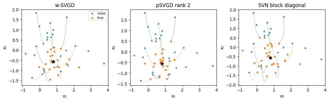
SVGD uses \(\phi(x)=N^{-1}\sum_j[k(x_j,x)\nabla\log\pi(x_j)+\nabla_{x_j}k(x_j,x)]\). We compare weight-space SVGD, likelihood-informed pSVGD and the published block-diagonal SVN approximation on a whitened Gaussian inverse problem; then transport predictions through an actual function map and destination VJP. R11, R12, R13, R14.

import os, json, time, platform
from pathlib import Path
import torch
import matplotlib.pyplot as plt
from IPython.display import display, Markdown
from lafa import samplers
from lafa.problems import Gaussian, GaussianMixture2D, Banana2D

torch.set_num_threads(1)
device = torch.device(os.environ.get('LAFA_DEVICE', 'cpu'))
if device.type == 'cuda' and not torch.cuda.is_available():
    raise RuntimeError('LAFA_DEVICE=cuda requested, but CUDA is unavailable')
dtype, seed = torch.float64, 2026
quick = os.environ.get('LAFA_QUICK', '1') == '1'
torch.manual_seed(seed)
def gen(offset=0):
    return torch.Generator(device=device).manual_seed(seed + offset)
def tensor(x): return torch.as_tensor(x, device=device, dtype=dtype)
def cpu(x): return x.detach().cpu().numpy()
def sync():
    if device.type == 'cuda': torch.cuda.synchronize(device)
def table(rows):
    keys = list(dict.fromkeys(k for row in rows for k in row))
    display(Markdown('| ' + ' | '.join(keys) + ' |\n|' + '|'.join(['---']*len(keys)) + '|\n' +
        '\n'.join('| ' + ' | '.join(f'{r[k]:.4g}' if isinstance(r.get(k),float) else str(r.get(k, '—')) for k in keys) + ' |' for r in rows)))
def contour(ax, target, bounds=(-5,5,-5,5)):
    a=torch.linspace(bounds[0],bounds[1],100,device=device,dtype=dtype)
    b=torch.linspace(bounds[2],bounds[3],100,device=device,dtype=dtype)
    xx,yy=torch.meshgrid(a,b,indexing='xy')
    with torch.no_grad(): u=target(torch.stack((xx,yy),-1))
    ax.contour(cpu(xx),cpu(yy),cpu(u-u.min()),levels=[.5,1,2,4,8,16],colors='0.7',linewidths=.6)
    ax.set(xlim=bounds[:2],ylim=bounds[2:]); ax.set_aspect('equal')
def covariance(x):
    z=x-x.mean(0); return z.T@z/(len(x)-1)
def collect(method, steps, burn=0, thin=1):
    samples=[]; trace=[]; hs=[]; accepted=[]
    for i in range(steps):
        r=method.step(); trace.append(r.position.reshape(-1,r.position.shape[-1])[0].clone())
        hs.append(float(torch.as_tensor(r.stats.get('step_size',getattr(method,'step_size',float('nan')))).double().mean()))
        if getattr(r,'accepted',None) is not None: accepted.append(r.accepted.double().mean())
        if i>=burn and (i-burn)%thin==0: samples.append(r.position.reshape(-1,r.position.shape[-1]))
    return torch.cat(samples),torch.stack(trace),hs,float(torch.stack(accepted).mean()) if accepted else float('nan')
root=Path.cwd() if (Path.cwd()/'docs').exists() else Path.cwd().parent
assets=root/'docs'/'assets'; assets.mkdir(parents=True,exist_ok=True)
print(json.dumps(dict(device=str(device),dtype=str(dtype),seed=seed,quick=quick,torch=torch.__version__,python=platform.python_version(),hardware=torch.cuda.get_device_name(device) if device.type=='cuda' else platform.processor() or platform.machine())))

{"device": "cpu", "dtype": "torch.float64", "seed": 2026, "quick": true, "torch": "2.6.0+cpu", "python": "3.12.14", "hardware": "x86_64"}

from lafa.particles import SVGD,ProjectedSVGD,SteinVariationalNewton,FunctionSpaceSVGD
from lafa.kernels import RBF
D,N=8,24; iterations=55 if quick else 200
x=torch.randn((N,D),device=device,dtype=dtype,generator=gen())
y=tensor([1.,-.7]); sigma=.5
def log_likelihood(z): return -.5*((z[...,:2]-y)/sigma).square().sum(-1)
def potential(z): return z.square().sum(-1)/2-log_likelihood(z)
mean=torch.zeros(D,device=device,dtype=dtype); mean[:2]=y/(1+sigma*sigma)
variance=torch.ones(D,device=device,dtype=dtype); variance[:2]=sigma*sigma/(1+sigma*sigma)
truth_cov=torch.diag(variance)
methods={'w-SVGD':SVGD(potential,x,step_size=.07,kernel=RBF(2.)),
 'pSVGD rank 2':ProjectedSVGD(log_likelihood,x,rank=2,step_size=.07,kernel=RBF(1.)),
 'SVN block diagonal':SteinVariationalNewton(potential,x,step_size=.025,kernel=RBF(2.),damping=.01,cg_max_iterations=30)}
paths={}; rows=[]
for name,m in methods.items():
    path=[m.position]; calls=0; sync(); start=time.perf_counter()
    for _ in range(iterations):
        r=m.step(); path.append(r.position); calls+=int(r.stats.get('cg_operator_calls',0))
    sync(); elapsed=time.perf_counter()-start; paths[name]=torch.stack(path)
    rows.append(dict(method=name,seconds=elapsed,mean_error=float((m.position.mean(0)-mean).norm()),covariance_error=float((covariance(m.position)-truth_cov).norm()),HVP_operator_calls=calls))
table(rows)

method	seconds	mean_error	covariance_error	HVP_operator_calls
w-SVGD	0.04784	0.1659	0.7152	0
pSVGD rank 2	0.04767	0.2899	1.073	0
SVN block diagonal	3.65	0.07341	0.6914	8052

fig,ax=plt.subplots(1,3,figsize=(11,3.3),layout='constrained')
for a,(name,path) in zip(ax,paths.items()):
    for k in range(min(N,12)): a.plot(cpu(path[:,k,0]),cpu(path[:,k,1]),lw=.6,alpha=.6)
    a.scatter(*cpu(path[0,:,:2]).T,s=10,marker='x',label='initial'); a.scatter(*cpu(path[-1,:,:2]).T,s=12,label='final')
    a.scatter(*cpu(mean[:2]),marker='*',s=80,color='k'); a.set_title(name); a.set(xlabel='x₁',ylabel='x₂')
ax[0].legend(fontsize=7); plt.show()
print('Projected likelihood basis residual:',float(methods['pSVGD rank 2'].basis_residual))

Projected likelihood basis residual: 9.39959687352353e-15

All methods use the same particles and iteration count, but SVN performs additional matrix-free curvature solves. Reported operator calls count block-operator evaluations, each of which can contain several target HVPs. pSVGD keeps the prior-distributed complement supplied at initialization; its frozen-complement profile score is an approximation, not an unbiased optimal-profile score. Finite deterministic particles are not independent MCMC draws.

# Finite function-space Bayesian polynomial regression.
t=torch.linspace(-1,1,15,device=device,dtype=dtype)
G=torch.stack((torch.ones_like(t),t,t.square()),-1)
yfun=.4+.7*t-.2*t.square()+.15*torch.randn(t.shape,device=device,dtype=dtype,generator=gen(40))
noise_sd=.25; prior_sd=2.
def fmap(w): return G@w
def fpotential(f): return .5*((f-yfun)/noise_sd).square().sum(-1)+.5*(f/prior_sd).square().sum(-1)
weights=torch.randn((24,3),device=device,dtype=dtype,generator=gen(41))*.4
fmethod=FunctionSpaceSVGD(fmap,fpotential,weights,step_size=.0008,kernel=RBF(1.5))
wmethod=SVGD(lambda w:fpotential(w@G.T),weights,step_size=.004,kernel=RBF(.5))
regression_steps=250 if quick else 1000
for _ in range(regression_steps): fmethod.step(); wmethod.step()
# Exact reference for the induced parameter density proportional to exp(-Uf(Gw)).
precision=(1/noise_sd**2+1/prior_sd**2)*(G.T@G)
cov=torch.linalg.inv(precision); mu=torch.linalg.solve(precision,G.T@yfun/noise_sd**2)
reference_mean=G@mu; reference_sd=(G@cov@G.T).diagonal().sqrt()
fig,ax=plt.subplots(1,2,figsize=(9,3.2),layout='constrained')
rows=[]
for a,(name,m) in zip(ax,[('weight coordinates',wmethod),('function coordinates + VJP',fmethod)]):
    predictions=m.position@G.T; pm=predictions.mean(0); sd=predictions.std(0)
    a.fill_between(cpu(t),cpu(pm-2*sd),cpu(pm+2*sd),alpha=.25,label='particle mean ±2 SD')
    a.plot(cpu(t),cpu(pm),label='particle mean'); a.plot(cpu(t),cpu(reference_mean),'k:',label='Gaussian reference')
    a.plot(cpu(t),cpu(reference_mean-2*reference_sd),'k:',lw=.6); a.plot(cpu(t),cpu(reference_mean+2*reference_sd),'k:',lw=.6)
    a.scatter(cpu(t),cpu(yfun),s=12); a.set_title(name); a.set(xlabel='input',ylabel='prediction')
    rows.append(dict(coordinates=name,predictive_mean_RMSE=float((pm-reference_mean).square().mean().sqrt()),predictive_SD_RMSE=float((sd-reference_sd).square().mean().sqrt())))
ax[0].legend(fontsize=7); plt.show(); table(rows)

coordinates	predictive_mean_RMSE	predictive_SD_RMSE
weight coordinates	0.001926	0.003511
function coordinates + VJP	0.004468	0.04507

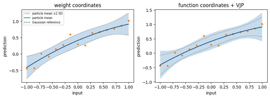
The fixed evaluation grid defines the function-space kernel and explicit function prior. The implementation maps each weight vector to predictions and pulls transport back with \(J_i^T\phi_i\). It is not an inverse-Jacobian step: induced prediction drift is \(J_iJ_i^T\phi_i\). A linear map is deliberately used so a Gaussian reference is available. Plotted ±2 SD bands summarize this finite ensemble; they are not calibrated coverage claims.

Batched neural-network parameters

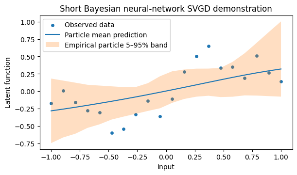
ModulePotential evaluates one full-data likelihood per parameter state. Chunked vmap matches explicit loop evaluation while bounding simultaneous activations. Here a Gaussian weight prior and the complete Gaussian observation likelihood define a small Bayesian neural network; the short SVGD run is an interacting approximation, so its particles are not inputs to independent-chain ESS or R-hat.

Use the target’s value_and_grad protocol when adding a prior to keep likelihood graphs bounded by the chunk size. A plain differentiable wrapper around likelihood(w) keeps each chunk’s graph until its later backward call.

from lafa.targets import ModulePotential
model = torch.nn.Sequential(torch.nn.Linear(1, 4), torch.nn.Tanh(), torch.nn.Linear(4, 1)).to(device=device, dtype=dtype).eval()
inputs = torch.linspace(-1, 1, 20, device=device, dtype=dtype)[:, None]
observed = .5 * torch.sin(3 * inputs) + .15 * torch.randn(inputs.shape, device=device, dtype=dtype, generator=gen(401))
loss = lambda prediction: .5 * ((prediction - observed) / .15).square().sum()
likelihood = ModulePotential(model, loss, args=(inputs,), chunk_size=8)
loop_likelihood = ModulePotential(model, loss, args=(inputs,), batch_mode='loop', chunk_size=8)
weights = torch.randn((32, likelihood.numel), device=device, dtype=dtype, generator=gen(402))
v, g = likelihood.value_and_grad(weights)
vl, gl = loop_likelihood.value_and_grad(weights)
torch.testing.assert_close(v, vl)
torch.testing.assert_close(g, gl)
class NeuralPosterior:
    def __call__(self, w):
        return likelihood(w) + .5 * w.square().sum(-1)

    def value_and_grad(self, w):
        # Evaluate/backpropagate one model chunk at a time, then add the prior.
        value, gradient = likelihood.value_and_grad(w)
        return value + .5 * w.square().sum(-1), gradient + w

ensemble = SVGD(NeuralPosterior(), weights, step_size=.001, kernel=RBF(2.), block_size=16)
for _ in range(60 if quick else 300): ensemble.step()
def predict(w):
    parameters = {s.name: w[s.start:s.stop].reshape(s.shape) for s in likelihood.parameter_spec}
    return torch.func.functional_call(model, parameters, (inputs,)).squeeze(-1)
with torch.no_grad(): predictions = torch.vmap(predict, chunk_size=8)(ensemble.position)
lo, hi = torch.quantile(predictions, tensor([.05, .95]), dim=0)
fig, ax = plt.subplots(figsize=(6, 3.5), layout='constrained')
ax.scatter(cpu(inputs[:, 0]), cpu(observed[:, 0]), s=15, label='Observed data')
ax.plot(cpu(inputs[:, 0]), cpu(predictions.mean(0)), label='Particle mean prediction')
ax.fill_between(cpu(inputs[:, 0]), cpu(lo), cpu(hi), alpha=.25, label='Empirical particle 5–95% band')
ax.set(xlabel='Input', ylabel='Latent function', title='Short Bayesian neural-network SVGD demonstration')
ax.legend(); plt.show()
print({'parameter_dimension': likelihood.numel, 'particles': len(weights), 'loop_vmap_max_gradient_error': float((g-gl).abs().max())})

{'parameter_dimension': 13, 'particles': 32, 'loop_vmap_max_gradient_error': 0.0}