2D full-waveform inversion in PyTorch
SimpleFWI is a Python research library for 2D, constant-density acoustic full-waveform inversion (FWI) in PyTorch. It models seismic data in the frequency domain with a Helmholtz solver, computes implicit adjoint gradients, and updates bounded velocity models with native PyTorch optimizers. The code is MIT licensed.
Start with the CPU sparse-direct reference solver. An experimental matrix-free CUDA FGMRES solver is available, with a recorded NVIDIA A40 validation run. The current examples establish small-problem integration and numerical parity; large-scale, high-frequency Marmousi recovery and GPU speedup remain unverified.
What can you do with SimpleFWI?
| Task | Implementation and next step |
|---|---|
| Model acoustic wavefields | Helmholtz equation with padded PML, optional pressure-release free surface |
| Invert several frequencies and grid resolutions | Coarse-to-fine and low-to-high continuation, physical squared-slowness transfer |
| Choose an optimizer | Native torch.optim recipes, including Adam, RMSprop and L-BFGS; 15 CPU recipes checked |
| Examine local uncertainty | Exact and Gauss–Newton Hessian-vector products, proper-prior local covariance actions |
| Record and reproduce a run | Accepted-state HDF5 recording and restart checkpoints, explicit configuration and dataset hashes |
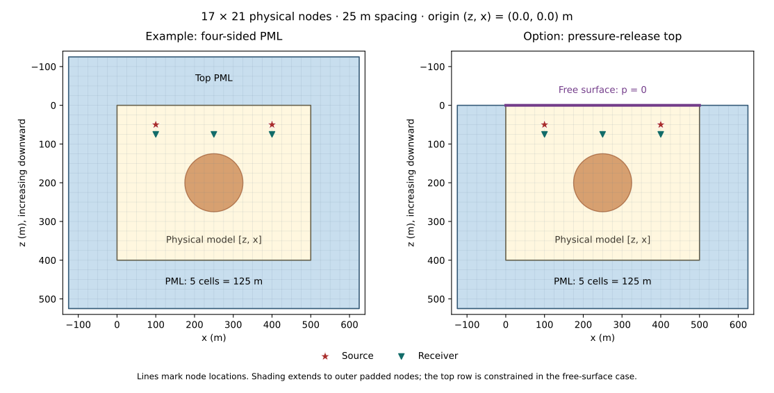
The illustration shows the complete README example geometry. The workflow is grid and acquisition → Helmholtz solve → receiver data → weighted misfit → adjoint gradient → optimizer update. Repeat the solves at the selected frequencies and model resolutions. Curvature and recording are explicit optional operations.
Install the validated CPU environment
Use Python 3.12 and PyTorch 2.12.0. From a fresh checkout:
git clone https://github.com/izzatum/SimpleFWI.git
cd SimpleFWI
python3.12 -m venv .venv
source .venv/bin/activate
python -m pip install torch==2.12.0 --index-url https://download.pytorch.org/whl/cpu
python -m pip install -r requirements/fwi2d-py312.lock
python -m pip install --no-deps -e '.[fwi2d]'
For NVIDIA CUDA, create a separate environment and select the matching official
PyTorch 2.12.0 CUDA wheel before installing the same lock file. The legacy
gpu-cuda extra is not the installation path for the PyTorch solver. Follow the
installation guide.
Run a small frequency-domain FWI example
From the installed checkout, use a new output path:
OPENBLAS_NUM_THREADS=1 OMP_NUM_THREADS=1 \
  python -m simplefwi.fwi2d --output /tmp/simplefwi-first-run
This runs a small Camembert integration example. Inspect the output manifest's
accuracy classification before interpreting the model. For a complete Python
example using AcousticFWI, VelocityParameters and InversionRunner, see the
executable README quickstart.
Models use SI units: metres, metres/second and Hz. Model arrays are [z, x];
observations are [frequency, source, receiver]. Defaults are float64 model
parameters, complex128 wavefields and the Fourier convention exp(-i omega t).
Learn with executable notebooks
- Helmholtz solver on CPU and GPU: Marmousi shows wavefields, residuals and explicit device comparisons.
- FWI with Adam, RMSprop and L-BFGS: Marmousi compares loss histories and measured computational work.
- Hessian and Gauss–Newton uncertainty: Camembert compares local curvature and proper-prior covariance on a small active window.
All three default notebooks have recorded CPU executions; the Helmholtz notebook also passed a separate bounded A40 execution. Read the validation record and FAQ for exact scope, numerical evidence and known limitations.
Cite and reproduce a result
Reference izzatum/SimpleFWI, retain the MIT license notice, and record the Git revision, configuration, data provenance, device, precision and solver tolerances used. No associated publication or DOI is claimed. For questions or reproducible bug reports, use GitHub issues.